Version 1.4.5
The ability to save data as a text file and to read it has been restored.
Version 1.4.4
The graphics functionality lost when using the Big Sur or higher operating system has been restored.
Version 1.4.3
Minor update with a new support site and a privacy statement
Version 1.4.2
Minor update.
Version 1.4.1
The program has been updated to a 64 bit application
Version 1.4.0
In this version the ability to read tab delimited text files has been added. The app icon has also undergone a minor revision.Version 1.3.0
In this version this version the ability to read csv files has been added. Therefore if an excel file is saved as a csv file, it can be opened via the file menu by selecting "Open csv file".Version 1.2.0
In this version you can delete an individual row from a data file you have created.
Version 1.1.0
The
application has been sandboxed and you now have the option to multiply
or divide x and/or y by a factor of your choice before linear
regression.
Description
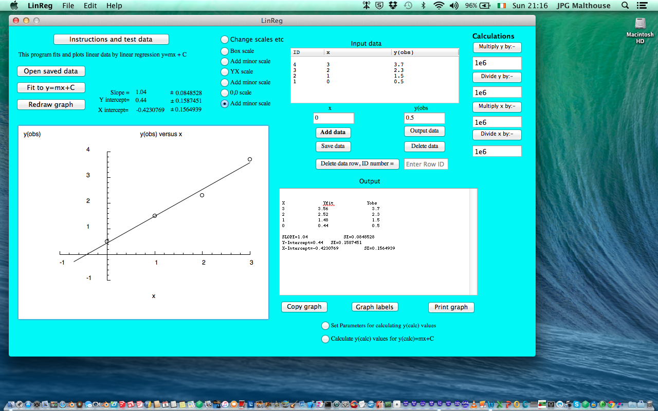
This program fits using linear regression and plots to the following equation:-y=mx+C
Three different scale types can be used. A box scale, a YX scale or y versus x scale and a 0,0 scale where both the y and x axes pass through zero.
Results can be saved, copied and pasted into other applications such as Word.
Please note, data points must be added individually. You CANNOT import data from other sources such as Excel. However, once you have inputted your data you can save it for future analysis.
FIRST INPUT DATA OR OPEN SAVED DATA
Buttons will be enabled as you need them.
Test data
x--- y
0----0.5
1----1.5
2--2.3
3----3.7
Enter data into the boxes "x" and "y"
Press button "Add Data"
Enter data into the boxes "x" and "y"
Select button "Add Data"
Repeat until all data is entered.
A minimum of 3 data points is required but preferably more points should be used.
Then you can save the data as a text file by selecting the "Save Data" button.
You can then reload the data at any time by selecting "Open Saved Data".
Selecting the "output data" button outputs data to the output window.
Alternatively if your data is in another program such as excel simply save it as a cvs file or as a Tab delimited text file.
If you then go to the File menu item you can select “Open cvs file” and you will be able to input data from the cvs file.
To input data saved as a Tab delimited text file go to the File menu and select “Open Tab file”.
TO ANALYZE DATA
Select "Fit to y=mx+C".
Answers for test data
SLOPE=1.04 SE=0.0848528
Y-Intercept=0.44 SE=0.1587451
X-Intercept=-0.4230769 SE=0.1564939
After selecting the required fit the analyzed data, fitted data and the fitted parameters will be outputted to the Output window. This output can be selected, printed or copied and pasted into other applications such as word. These options will be found under the File and Edit menus.
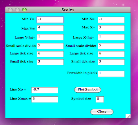
Then select the type of scale you require.
Select "Change scales etc" and enter the changes you require. After changing the graph scales, press redraw to implement the changes.
You do not need to make changes for the test data just close the"Change scales etc" window and select "Redraw". This is a good time to try out the different scales Box, YX and 0,0. The 0,0 scale allows you to plot graphs with both the x and y axes passing through zero.
To give the graph a title and label the axes, select "Graph labels" and make the appropriate changes.
AFTER CHANGING THE GRAPH SCALES OR LABELS, PRESS "REDRAW" TO IMPLEMENT THE CHANGES.
Select "Copy graph" to copy the graph to the clipboard. You may then paste it into other applications such as Word.
Select "Print graph" to output the graph to your printer.
If you want to calculate theoretical data you can select "Set parameters for calculating kobs values", enter values, then select "Calculate y(calc) values for y(calc)=mx+C" to output the data to the output window.